Diffusion models are a class of probabilistic models that generate data by iteratively refining a noisy sample until it resembles the target data.
The Core Concept: Diffusion and Denoising
At the heart of diffusion models are two processes: diffusion and denoising.
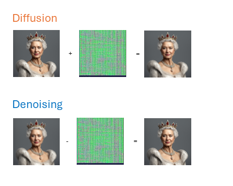
Diffusion: This is a forward process where data (e.g., an image) is gradually corrupted by adding noise over several steps. Imagine starting with a clear image and progressively adding layers of random noise until it becomes almost unrecognizable.
Denoising: This is the reverse process, where the model learns to gradually remove noise from the corrupted data, step by step, to recover the original data distribution. The model is trained to predict and subtract the noise at each step, refining the noisy data back to a high-quality sample.
The Steps in Diffusion Models
- Forward Diffusion Process: The model takes a data sample (e.g., an image) and corrupts it by adding Gaussian noise incrementally over a series of steps. Each step is a small perturbation, leading to a fully noisy sample at the end of the process. This follows a Markov chain, where each state of the image depends solely on the state from the previous step, not on any earlier steps.
- Gaussian noise: It changes the pixel values of an image so that the image becomes corrupted.
- Reverse Denoising Process: The model is trained to reverse the diffusion process. Starting from the noisy sample, the model uses a neural network to predict the noise added at each step and subtract it, progressively denoising the sample until it resembles the original data.
- Loss Function: During training, the model minimizes the difference between the predicted noise and the actual noise added during the forward process. This typically involves optimizing a loss function that measures this discrepancy such as MSE loss. The MSE loss measures the discrepancy between the noise we randomly define (don't think about noise as a singular value; it is also a matrix like an image) and the input image with noise introduced. So in such a way, we train our model to recognize noise in the image.
- Sampling: Once trained, the model can generate new samples by starting from a random noise vector and applying the learned denoising steps in reverse order.